Correlation Coefficient with SigmaXL

Pearson’s Correlation Coefficient

Pearson’s correlation coefficient is also called Pearson’s r or coefficient of correlation and Pearson’s product moment correlation coefficient (r), where r is a statistic measuring the linear relationship between two variables.

What is Correlation?

Correlation is a statistical technique that describes whether and how strongly two or more variables are related.
Correlation analysis helps to understand the direction and degree of association between variables, and it suggests whether one variable can be used to predict another. Of the different metrics to measure correlation, Pearson’s correlation coefficient is the most popular. It measures the linear relationship between two variables.
Correlation coefficients range from −1 to 1.

• If r = 0, there is no linear relationship between the variables.
• The sign of r indicates the direction of the relationship:
• If r < 0, there is a negative linear correlation. If r > 0, there is a positive linear correlation.
  The absolute value of r describes the strength of the relationship:
• If |r| ≤ 0.5, there is a weak linear correlation.
• If |r| > 0.5, there is a strong linear correlation.
• If |r| = 1, there is a perfect linear correlation.
  When the correlation is strong, the data points on a scatter plot will be close together (tight). The closer r is to −1 or 1, the stronger the relationship.
• −1 Strong inverse relationship
• +1 Strong direct relationship
  When the correlation is weak, the data points are spread apart more (loose). The closer the correlation is to 0, the weaker the relationship.

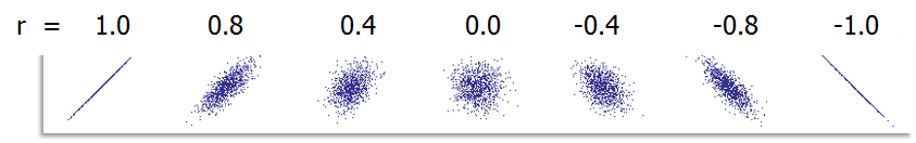Fig 1.0 Examples of Types of Correlation

This Figure demonstrates the relationships between variables as the Pearson r value ranges from 1 to 0 and to −1. Notice that at −1 and 1 the points form a perfectly straight line.

• At 0 the data points are completely random.
• At 0.8 and −0.8, notice how you can see a directional relationship, but there is some noise around where a line would be.
• At 0.4 and −0.4, it looks like the scattering of data points is leaning to one direction or the other, but it is more difficult to see a relationship because of all the noise.

Pearson’s correlation coefficient is only sensitive to the linear dependence between two variables. It is possible that two variables have a perfect non-linear relationship when the correlation coefficient is low. Notice the scatter plots below with correlation equal to 0. There are clearly relationships but they are not linear and therefore cannot be determined with Pearson’s correlation coefficient.

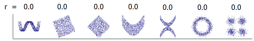Fig 1. 1 Examples of Types of Relationships

Correlation and Causation

Correlation does not imply causation.
If variable A is highly correlated with variable B, it does not necessarily mean A causes B or vice versa. It is possible that an unknown third variable C is causing both A and B to change. For example, if ice cream sales at the beach are highly correlated with the number of shark attacks, it does not imply that increased ice cream sales cause increased shark attacks. They are triggered by a third factor: summer.
This example demonstrates a common mistake that people make: assuming causation when they see correlation. In this example, it is hot weather that is a common factor. As the weather is hotter, more people consume ice cream and more people swim in the ocean, making them susceptible to shark attacks.

Correlation and Dependence

If two variables are independent, the correlation coefficient is zero.
WARNING! If the correlation coefficient of two variables is zero, it does not imply they are independent. The correlation coefficient only indicates the linear dependence between two variables. When variables are non-linearly related, they are not independent of each other but their correlation coefficient could be zero.

Correlation Coefficient and X-Y Diagram

The correlation coefficient indicates the direction and strength of the linear dependence between two variables but it does not cover all the existing relationship patterns. With the same correlation coefficient, two variables might have completely different dependence patterns. A scatter plot or X-Y diagram can help to discover and understand additional characteristics of the relationship between variables. The correlation coefficient is not a replacement for examining the scatter plot to study the variables’ relationship.
The correlation coefficient by itself does not tell us everything about the relationship between two variables. Two relationships could have the same correlation coefficient, but completely different patterns.

Statistical Significance of the Correlation Coefficient

The correlation coefficient could be high or low by chance (randomness). It may have been calculated based on two small samples that do not provide good inference on the correlation between two populations.
In order to test whether there is a statistically significant relationship between two variables, we need to run a hypothesis test to determine whether the correlation coefficient is statistically different from zero.
Hypothesis Test Statements

• H₀: r = 0: Null Hypothesis: There is no correlation.
• H1: r ≠ 0: Alternate Hypothesis: There is a correlation.

Hypothesis tests will produce p-values as a result of the statistical significance test on r. When the p-value for a test is low (less than 0.05), we can reject the null hypothesis and conclude that r is significant; there is a correlation. When the p-value for a test is > 0.05, then we fail to reject the null hypothesis; there is no correlation.
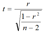
We can also use the t statistic to draw the same conclusions regarding our test for significance of the correlation coefficient. To use the t-test to determine the statistical significance of the Pearson correlation, calculate the t statistic using the Pearson r value and the sample size, n.
Test Statistic

Critical Statistic
Is the t-value in t-table with (n – 2) degrees of freedom.
If the absolute value of the calculated t value is less than or equal to the critical t value, then we fail to reject the null and claim no statistically significant linear relationship between X and Y.

• If |t| ≤ t_critical, we fail to reject the null. There is no statistically significant linear relationship between X and Y.
• If |t| > t_critical, we reject the null. There is a statistically significant linear relationship between X and Y.

Using Software to Calculate the Correlation Coefficient

We are interested in understanding whether there is linear dependence between a car’s MPG and its weight and if so, how they are related. The MPG and weight data are stored in the “Correlation Coefficient” tab in “Sample Data.xlsx.” We will discuss three ways to get the results.

Use Excel to Calculate the Correlation Coefficient

The formula CORREL in Excel calculates the sample correlation coefficient of two data series. The correlation coefficient between the two data series is −0.83, which indicates a strong negative linear relationship between MPG and weight. In other words, as weight gets larger, gas mileage gets smaller.

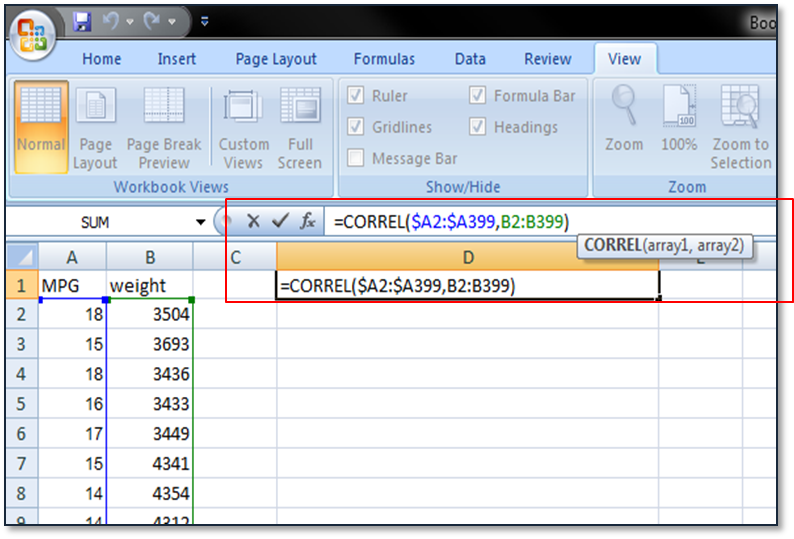
Fig 1.3 Correlation coefficient in Excel

 Interpreting Results

How do we interpret results and make decisions based Pearson’s correlation coefficient (r) and p-values?
Let us look at a few examples:

• r = −0.832, p = 0.000 (previous example). The two variables are inversely related and the linear relationship is strong. Also, this conclusion is significant as supported by p-value of 0.00.
• r = −0.832, p = 0.71. Based on r, you should conclude the linear relationship between the two variables is strong and inversely related. However, with a p-value of 0.71, you should then conclude that r is not significant and that your sample size may be too small to accurately characterize the relationship.
• r = 0.5, p = 0.00. Moderately positive linear relationship, r is statistically significant.
• r = 0.92, p = 0.61. Strong positive linear relationship but r is not statistically significant. Get more data.
• r = 1.0, p = 0.00. The two variables have a perfect linear relationship and r is significant.

Correlation Coefficient Calculation

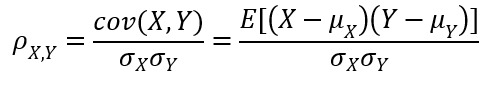
Population Correlation Coefficient (ρ)

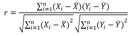
Sample Correlation Coefficient (r)

It is only defined when the standard deviations of both X and Y are non-zero and finite. When covariance of X and Y is zero, the correlation coefficient is zero.