Logistic Regression with SigmaXL

What is Logistic Regression?

Logistic regression is a statistical method to predict the probability of an event occurring by fitting the data to a logistic curve using logistic function. The regression analysis used for predicting the outcome of a categorical dependent variable, based on one or more predictor variables. The logistic function used to model the probabilities describes the possible outcome of a single trial as a function of explanatory variables. The dependent variable in a logistic regression can be binary (e.g. 1/0, yes/no, pass/fail), nominal (blue/yellow/green), or ordinal (satisfied/neutral/dissatisfied). The independent variables can be either continuous or discrete.

Logistic Function

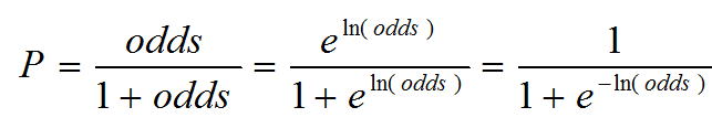
Where: z can be any value ranging from negative infinity to positive infinity.
The value of f(z) ranges from 0 to 1, which matches exactly the nature of probability (i.e., 0 ≤ P ≤ 1).
Logistic Regression Equation
Based on the logistic function,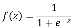

we define f(z) as the probability of an event occurring and z is the weighted sum of the significant predictive variables.

Where: Z represents the weighted sum of all of the predictive variables.

Logistic Regression

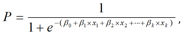
Another of way of representing f(z) is by replacing the z with the sum of the predictive variables.

Where: Y is the probability of an event occurring and x’s are the significant predictors.
Notes:

[unordered_list style=”star”]

• When building the regression model, we use the actual Y, which is discrete (e.g. binary, nominal, ordinal).
• After completing building the model, the fitted Y calculated using the logistic regression equation is the probability ranging from 0 to 1. To transfer the probability back to the discrete value, we need SMEs’ inputs to select the probability cut point.

[/unordered_list]

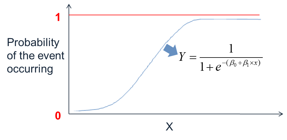
Logistic Curve

The logistic curve for binary logistic regression with one continuous predictor is illustrated by the following Figure.

Odds

Odds is the probability of an event occurring divided by the probability of the event not occurring.

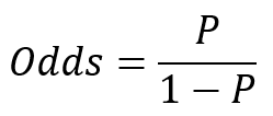
Odds range from 0 to positive infinity.
Probability can be calculated using odds.

Because probability can be expressed by the odds, and we can express probability through the logistic function, we can equate probability, odds, and ultimately the sum of the independent variables.
Since in logistic regression model

therefore

Three Types of Logistic Regression

[unordered_list style=”star”]

• Binary Logistic Regression
  • Binary response variable
  • Example: yes/no, pass/fail, female/male
• Nominal Logistic Regression
  • Nominal response variable
  • Example: set of colors, set of countries
• Ordinal Logistic Regression
  • Ordinal response variable
  • Example: satisfied/neutral/dissatisfied

[/unordered_list]

All three logistic regression models can use multiple continuous or discrete independent variables and can be developed in SXL using the same steps.

How to Run a Logistic Regression in SigmaXL

We want to build a logistic regression model using the potential factors to predict the probability that the person measured is female or male.

Data File: “Logistic Regression” tab in “Sample Data.xlsx”

Response and Potential Factors

[unordered_list style=”star”]

• Response (Y): Female/Male
• Potential Factors (Xs):
  • Age
  • Weight
  • Oxy
  • Runtime
  • RunPulse
  • RstPulse
  • MaxPulse

[/unordered_list]

Step 1:

1. Select the entire range of data (“Name”, “Sex”, “Age”, “Weight”, “Oxy”, “Runtime”, “RunPulse”, “RstPulse”, “MaxPulse” columns)
2. Click SigmaXL -> Statistical Tools -> Regression ->Binary Logistic Regression
3. A new window named “Binary Logistic Regression” appears with the selected range of data appearing in the box under “Please select your data”
   
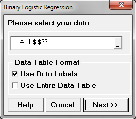
4. Click “Next>>”
5. A new window also called “Binary Logistic Regression” pops up.
6. Select “Sex” as the “Binary Response (Y)”
   Select “Age”, “Weight”, “Oxy”, “Runtime”, “RunPulse”, “RstPulse”, “MaxPulse” as the “Continuous Predictors (X)”.
   
   
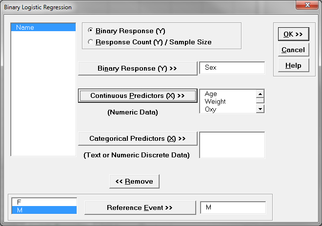
7. The reference event is set as “M” by default.
8. Click “OK”

Step 2:

1. Check the p-values of all the independent variables in the model.
2. Remove the insignificant independent variable one at a time from the model and rerun the model.
3. Repeat step 2.1 until all of the independent variables in the model are statistically significant.
   

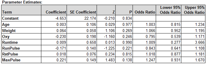
Since the p-values of all the independent variables are higher than the alpha level (0.05), we need to remove the insignificant independent variables one at a time from the model, starting from the one with the highest p-value. Runtime has the highest p-value (0.9897), so it would be removed from the model first. Re-run the binary logistic regression but this time exclude Runtime from the “Continuous Predictors (X)” in the Binary Logistic Regression dialog box.
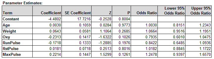After removing Runtime from the model, the p-values of all the independent variables are still higher than the alpha level (0.05). We need to continue removing the insignificant independent variables one at a time from the model, starting from the one with the highest p-value. Age has the highest p-value (0.9773), so it would be removed from the model next.

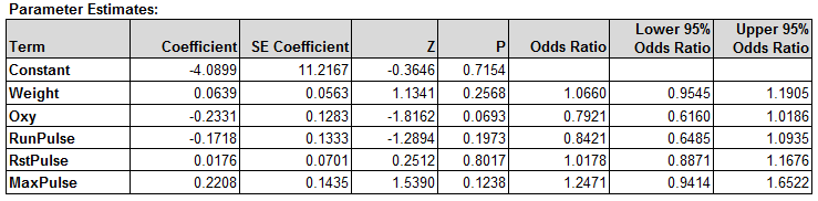After removing Age from the model, the p-values of all the independent variables are still higher than the alpha level (0.05). We need to continue removing the insignificant independent variables one at a time from the model, starting from the one with the highest p-value. RstPulse has the highest p-value (0.8017) so it would be removed from the model next.

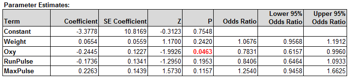After removing RstPulse from the model, the p-values of all the independent variables are still higher than the alpha level (0.05). We need to continue removing the insignificant independent variables one at a time from the model, starting from the one with the highest p-value. Weight has the highest p-value (0.242), so it would be removed from the model next.
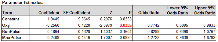After removing Weight from the model, the p-values of all the independent variables are still higher than the alpha level (0.05). We need to continue removing the insignificant independent variables one at a time from the model, starting from the one with the highest p-value. RunPulse has the highest p-value (0.1604), so it would be removed from the model next.
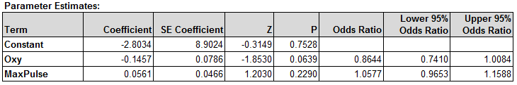After removing RunPulse from the model, the p-values of all the independent variables are still higher than the alpha level (0.05). We need to continue removing the insignificant independent variables one at a time from the model, starting from the one with the highest p-value. MaxPulse has the highest p-value (0.2290), so it would be removed from the model next.
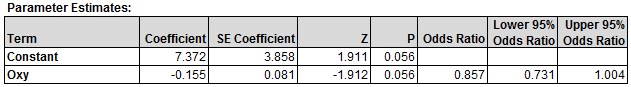After removing MaxPulse from the model, the p-value of the only remaining independent variable “Oxy” is at the alpha level (0.05). There is no need to remove “Oxy” from the model, we will accept the minute risk of rejecting the null at this p-value (0.0556). But before we do that, let’s check the validity of the model as a whole.

Step 3:

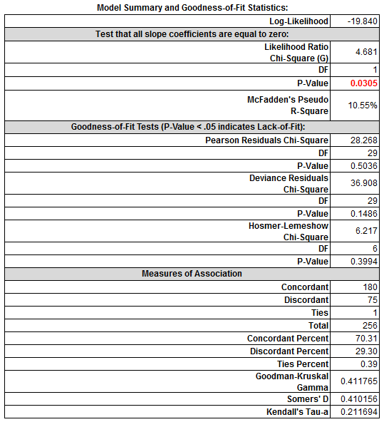
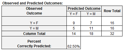
Analyze the binary logistic report and check the performance of the logistic regression model. The p-value here is greater than the alpha level of (0.05). We will conclude that at least one of the slope coefficients is not equal to zero. The pseudo R-squared is 10.55%. The R-squared of logistic regression is in general lower than the R-squared of the traditional multiple linear regression model. The p-value of lack of fit test is higher than alpha level (0.05). We conclude that the model fits the data. Also, 62.50% of the predicted outcomes match the observed outcomes.

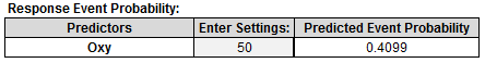
Step 4: Enter the setting of the Oxy into the cell highlighted in yellow and the predicted event probability would appear automatically. In this case, if we set the oxy value to 50, the probability that the person measured being male is 41%.