


One Sample t Test with SigmaXL
What is a One Sample t Test?
A One sample t test is a hypothesis test to study whether there is a statistically significant difference between a population mean and a specified value.
[unordered_list style=”star”]
- Null Hypothesis (H0): μ = μ0
- Alternative Hypothesis (Ha): μ ≠ μ0
[/unordered_list]
Where:
[unordered_list style=”star”]
- μ is the mean of a population of our interest
- μ0 is the specific value we want to compare against.
[/unordered_list]
What is a t-Test?
In statistics, a t-test is a hypothesis test in which the test statistic follows a Student’s t distribution if the null hypothesis is true. We apply a t-test when the population variance (σ) is unknown and we use the sample standard deviation (s) instead. A hypothesis test is a statistical method in which a specific hypothesis is formulated about a population, and the decision of whether to reject the hypothesis is made based on sample data. Hypothesis tests help to determine whether a hypothesis about a population or multiple populations is true with certain confidence level based on sample data. Hypothesis testing is a critical tool in the Six Sigma tool belt. It helps us separate fact from fiction, and special cause from noise, when we are looking to make decisions based on data.
Assumptions of One Sample t Test
- The sample data of the population of interest are unbiased and representative.
- The data of the population are continuous.
- The data of the population are normally distributed.
- The variance of the population of our interest is unknown.
- One sample t-test is more robust than the z-test when the sample size is small (< 30).
Normality Test
To check whether the population of our interest is normally distributed, we need to run normality test. While there are many normality tests available, such as Anderson–Darling, Sharpiro–Wilk, and Jarque–Bera, our examples will default to using the Anderson-Darling test for normality.
[unordered_list style=”star”]
- Null Hypothesis (H0): The data are normally distributed.
- Alternative Hypothesis (Ha): The data are not normally distributed.
[/unordered_list]
Test Statistic and Critical Value of One Sample t Test
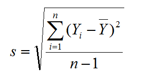
To understand what is happening when you run a t-test with your software, the formulas here will walk you through the key calculations and how to determine if the null hypothesis should be accepted or rejected. To determine significance, you must calculate the t-statistic and compare it to the critical value, which is a reference value based on the alpha value and degrees of freedom (n – 1). The t-statistic is calculated based on the sample mean, the sample standard deviation, and the sample size.
Test statistic is calculated with the formula:
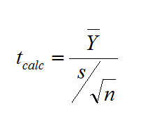
(Y ) ̅is the sample mean, n is the sample size, and s is the sample standard deviation
Critical value
[unordered_list style=”star”]
- tcrit is the t-value in a Student’s t distribution with the predetermined significance level α and degrees of freedom (n –1).
- tcrit values for a two-sided and a one-sided hypothesis test with the same significance level α and degrees of freedom (n – 1) are different.
[/unordered_list]
Decision Rules of One Sample T-Test
Based on the sample data, we calculated the test statistic tcalc, which is compared against tcrit to make a decision of whether to reject the null.
[unordered_list style=”star”]
- Null Hypothesis (H0): μ = μ0
- Alternative Hypothesis (Ha): μ ≠ μ0
[/unordered_list]
If |tcalc| > tcrit, we reject the null and claim there is a statistically significant difference between the population mean μ and the specified value μ0.
If |tcalc| < tcrit, we fail to reject the null and claim there is not any statistically significant difference between the population mean μ and the specified value μ0.
Use SigmaXL to Run a One Sample t Test
Case study: We want to compare the average height of basketball players against 7 feet.
Data File: “One Sample T-Test” tab in “Sample Data.xlsx”
[unordered_list style=”star”]
- Hypothesis (H0): μ = 7
- Alternative Hypothesis (Ha): μ ≠ 7
[/unordered_list]
Step 1: Test whether the data are normally distributed
- Select the entire range of data
- Click SigmaXL -> Graphical Tools -> Histograms & Descriptive Statistics
- A new window named “Histograms & Descriptive” pops up with the selected range appearing in the box under “Please select your data”
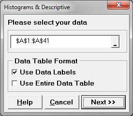
- Click “Next>>”
- A new window named “Histograms & Descriptive Statistics” appears
- Select “HtBk” as the “Numeric Data Variables (Y)”
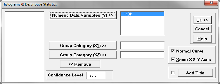
- Click “OK”
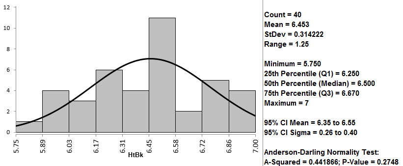
- The normality test results appear in the newly generated tab “Hist Descript (1)”
[unordered_list style=”star”]
- Null Hypothesis(H0): The data are normally distributed.
- Alternative Hypothesis(Ha): The data are not normally distributed.
[/unordered_list]
Since the p-value of the normality is 0.275, which is greater than alpha level (0.05), we fail to reject the null and claim that the data are normally distributed. If the data are not normally distributed, you need to use hypothesis tests other than the one sample t-test.
Now we can run the one-sample t-test, knowing the data are normally distributed.
Step 2: Run the one-sample t-test
- Select the entire range of “HtBk”
- Click SigmaXL -> Statistical Tools -> 1 Sample t-Test & Confidence Intervals
- A new window named “1 Sample t-Test” pops up with the selected range pre-populated in the box under “Please select your data”

- Click “Next>>”
- Another window also named “1 Sample t-Test” appears
- Select the radio button for “Unstacked Column Format”
- Select “HtBk” as the “Numerical Data Variable (Y)”
- Enter the hypothesized value “7” into the box next to “H0: Mean =”
- Select “Not Equal To” in the box next to “Ha:”
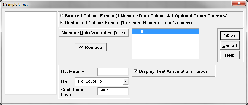
- Click “OK>>”
- The one-sample t-test result appears automatically in the tab “1 Sample t-Test (1)”.
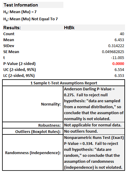
Model summary: Since the p-value is smaller than alpha level (0.05), we reject the null hypothesis and claim that average of basketball players is statistically different from 7 feet.