Paired t Test with SigmaXL

Paired t Test

The third type of a Two Sample t-Test is the Paired t Test.  This test is used when the two populations are dependent of each other, so each data point from one distribution corresponds to a data point in the other distribution. When using a paired t test, the test statistic is calculated using the average difference between the data pairs, the standard deviation of the differences, and the sample size of either population.

Test Statistic

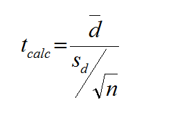
Where:

[unordered_list style=”star”]

• d is the difference between each pair of data
• is the average of d
• n is the sample size of either population of interest

[/unordered_list]

Critical Value

[unordered_list style=”star”]

• t_crit is the t value in a Student’s t distribution with the predetermined significance level α and degrees of freedom (n – 1).
• t_crit values for a two-sided and a one-sided t-test with the same significance level α and degrees of freedom (n – 1) are different.

[/unordered_list]

The critical t is looked up using the significance level alpha and degrees of freedom (n – 1).

Use SigmaXL to run a Paired t Test

Case study: We are interested to know whether the average salaries ($1000/yr.) of male and female professors at the same university are the same.
Data File: “Paired T-Test” tab in “Sample Data.xlsx”

The data were randomly collected from 22 universities. For each university, the salaries of male and female professors were randomly selected.

[unordered_list style=”star”]

• Null Hypothesis (H0): μmale – μfemale = 0
• Alternative Hypothesis (Ha): μmale – μfemale ≠ 0

[/unordered_list]

Step 1: Test whether the difference is normally distributed.

[unordered_list style=”star”]

• Null Hypothesis (H₀): The difference between two data sets is normally distributed.
• Alternative Hypothesis (H_a): The difference between two data sets is not normally distributed.

[/unordered_list]

1. Select the entire range of “Difference”
2. Click SigmaXL -> Graphical Tools -> Histograms & Descriptive Statistics
3. A new window named “Histogram & Descriptive” pops up with the selected range pre-populated in the box under “Please select your data”
   
4. Click “Next>>”
5. A new window named “Histograms & Descriptive Statistics” appears.
6. Select “Difference” as the “Numeric Data Variables (Y)”
   
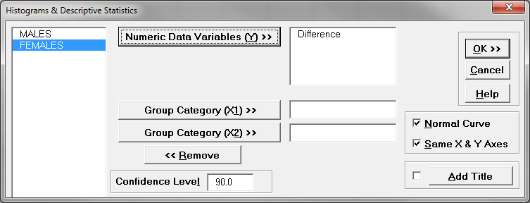
7. Click “OK>>”
8. The results of the Normality Test show in the tab “Hist Descript (1)”
   

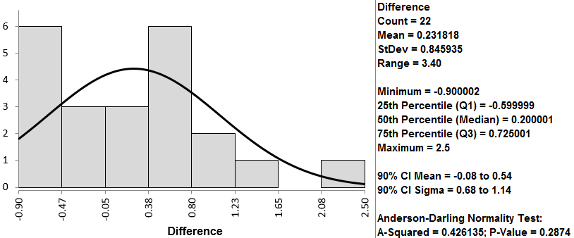
The p-value of the normality test is 0.287, greater than the alpha level (0.05), so we fail to reject the null hypothesis and we claim that the difference is normally distributed. When the difference is not normally distributed, we need other hypothesis testing methods.

Step 2: Run the paired t-test to compare the means of two dependent data sets.

1. Select the entire range of both MALES and FEMALES data
2. Click SigmaXL -> Statistical Tools -> Paired t-Test
3. A new window named “Paired t-Test” pops up with the selected range pre-populated in the box under “Please select your data”
   
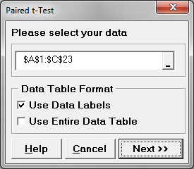
4. Click “Next >>”
5. Another new window named “Paired t-Test” pops up
6. Select “MALES” as “Numeric Data Variable 1”
   Select “FEMALES” as “Numeric Data Variable 2”
   
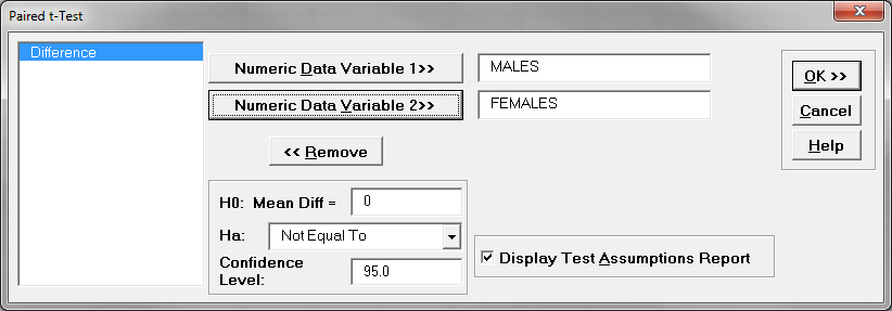
7. Click “OK>>”
8. The paired t-test results appear in the tab “Paired t-Test (1)”
   

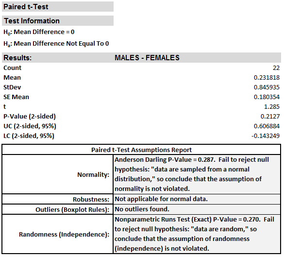
Model summary: The p-value of the paired t-test is 0.213, greater than the alpha level (0.05), so we fail to reject the null hypothesis and we claim that there is no statistically significant difference between the salaries of male and those of female professors. Because the p-value is higher than 0.05, we again fail to reject the null hypothesis, meaning that there is no statistically significant difference between the salaries of male and female professors.